7-clusters scatter
For visualization of 7-cluster structure a data set for every 143 genome was prepared in the following way:
1) A Genbank file with full genome was downloaded from Genbank FTP-site. Using BioJava package the complete sequence and the annotation was parsed. In the case when the genome had two chromosomes, the sequences of both were concantenated. The short sequences of plasmids were ignored.
2) We have sequence ![]() having length
having length ![]() and
and ![]() is a letter in
the
is a letter in
the ![]() th position of
th position of ![]() . We define a constant
. We define a constant ![]() , window size
, window size
![]() and in every position
and in every position ![]() ,
,
![]() , we open
a window in the sequence, centered in position
, we open
a window in the sequence, centered in position ![]() . In every
window we count words of length
. In every
window we count words of length ![]() , starting from every third
position:
, starting from every third
position:
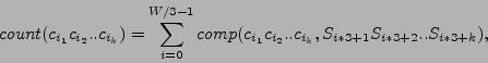 |
(1) |
where
![]() is string comparison function having
value 1 if
is string comparison function having
value 1 if ![]() equals
equals ![]() and 0 otherwise.
and 0 otherwise. ![]() is a
letter from genetic alphabet (
is a
letter from genetic alphabet (![]() ,
, ![]() ,
, ![]() ,
, ![]() ).
).
For every window a frequency vector is defined:
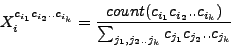 |
(2) |
All words containing non-standard letters like N, S, W are ignored.
The data set ![]() ,
,
![]() is normalized to
have unity standard deviation and zero mean.
is normalized to
have unity standard deviation and zero mean.
3) Using annotation from Genbank file for every window a label is assigned accordingly to if the center of window is inside a marked CDS feture (including hypothetical ones) or not. In the first case the reading frame and the strand of the CDS feature are determined and the window is assigned one of F0,F1,F2,B0,B1,B2 lable. In the second case the label is J.
4) A standard PCA-analysis is performed and the first three
principal components are calculated. They form form a
3D-orthonormal basis in ![]() -dimensional space. Every point is
projected in the basis, thus we assign three coordinates for every
point .
-dimensional space. Every point is
projected in the basis, thus we assign three coordinates for every
point .
7cluster schema
To create the schema of 7-cluster structure the following method
was utilized. We calculated the mean point ![]() for every subset
with a given label
for every subset
with a given label ![]() .
.
For the set of centroids ![]() ,
, ![]() ,
, ![]() ,
, ![]() ,
,
![]() ,
, ![]() a distance matrix of euclidean distances was
calculated and visualized using classical MDS.
a distance matrix of euclidean distances was
calculated and visualized using classical MDS.
To visualize the "radii" of the subsets, a mean squared distance
![]() to the centroid
to the centroid ![]() was calculated (intraclass dispersion).
To visualize the value on 2D plane, we have to introduce dimension
correction factor, so the radius drawn on the picture equals
was calculated (intraclass dispersion).
To visualize the value on 2D plane, we have to introduce dimension
correction factor, so the radius drawn on the picture equals
 |
(3) |
The form of the cluster is not always spherical and often
intersection of radii do not reflect real overlapping of classes
in high-dimensional space. To show how good the classes are
separated in fact, we developped the following method for cluster
contour visualization. To create a contour for class ![]() , we
calculate averages of all positive and negative projections on the
vectors connecting centroid
, we
calculate averages of all positive and negative projections on the
vectors connecting centroid ![]() and 6 other centroids
and 6 other centroids ![]() .
.
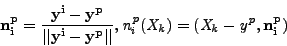 |
(4) |
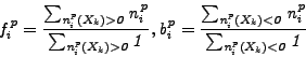 |
(5) |
Then, using the 2D MDS plot where every vector ![]() has 2
coordinates, we put 12 points
has 2
coordinates, we put 12 points ![]() ,
, ![]() analogously.
analogously.
 |
(6) |
| (7) |
Using a smoothing procedure in polar coordinates we create a smooth contour approximating these 12 points.